As part of getting my wisdom teeth removed a few years ago, I had a CT scan of my jaw done to see where my wisdom teeth were and at what angle. I can only describe the agle they turned out to be as hilariously incorrect.

Anyway, a CT scan works by taking a bunch of 2D x-ray images from many angles. Each of those 2D images encodes information about the density of all the tissues that the beam had to pass through on the way from the source to the detector for that pixel. Using the magic of the Radon transform, you can take that collection of 2D images and compute a 3D density map of, in this case, my head.

Being the nerd that I am, I asked if I could have the scan data and they very kindly burned it to a CD for me. At some point in the intervening years I copied the data from the CD to ‘my various files I might need at some point’ place and forgot about it.

Since I’ve been playing around a lot with three.js lately I wondered how hard it would be to finally visualise the scan.

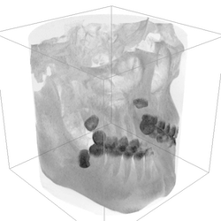
So as not to bury the lede, here’s what I currently have:

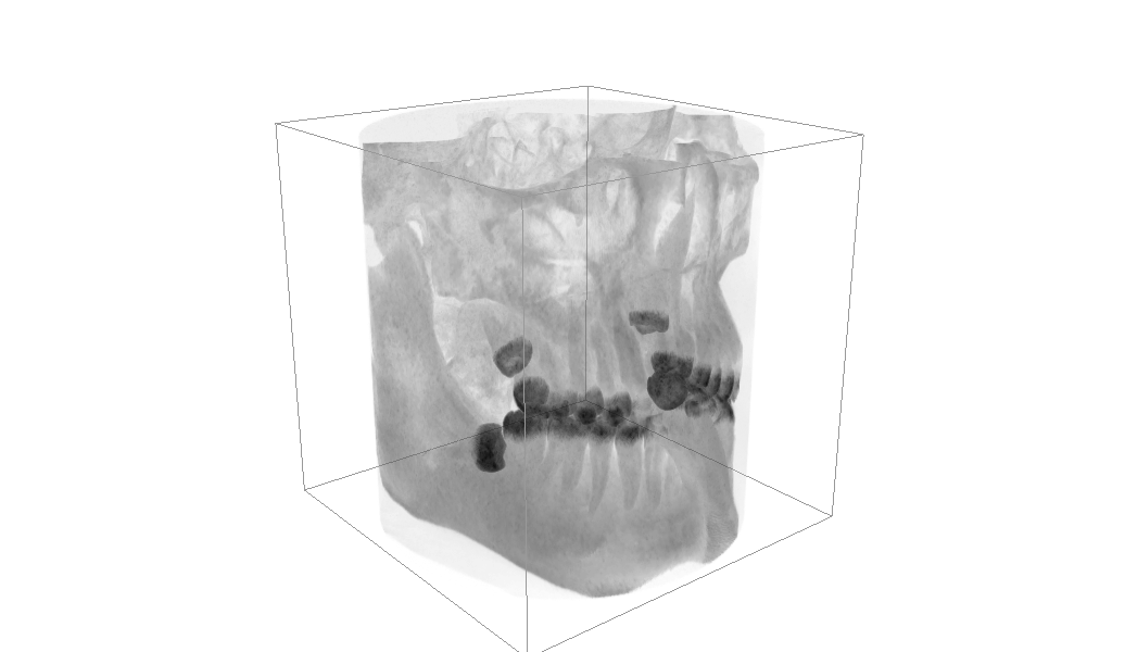
Open the settings to control the render mode, a ray is shot out from the camera through each pixel then through the volume: Max Intensity: each pixel is coloured based on the densest voxel it passed through. Mean Intensity: instead use the mean, ignoring empty space. Min Intensity: same but use the minimum ignoring empty space. IsoSurface: Only consider data with within a certain width around a particular value.

The default view should show my bones and teeth quite well, if you hit presets and choose “Air Pockets” you can just about see the outline of where the various air pockets inside my head are. Also my tongue for some reason.

Read on if you want to know the techy side of how I put this together.

Step 1: Extracting the data

The file on the CD was in a .inv3 format. A quick google sent me to this page with a nice explanation of the file format. It turns out it was encoded with an open source tool! Now I could probably have just installed InVesalius and exported the data that way but instead I went with just reading the file which was pretty easy because they chose quite a simple format.

First step was to extract it:

tar -xvzf my_scan.inv3

which gave me these file:

4.0K        main.plist
130M        mask_0.dat
4.0K        mask_0.plist
258M        matrix.dat
4.0K        measurements.plist
4.0K        surface_0.plist
101M        surface_0.vtp
4.0K        surface_1.plist
3.9M        surface_1.vtp
... more pairs of surface_n.vtp and surface_n.plist
4.0K        surface_8.plist
4.4M        surface_8.vtp

From my quick skim of the file format page, main.plist has the main metadata, matrix.dat is the density data. I think mask_n.dat and mask.plist are basically an array of indices used to categorise each pixel in the raw scan, for example bone, soft tissue etc. I think all the surface_n.* pairs and the mask might be from when I was playing around with the tools inside InVesalius sometime in the distant past.

For the rest of this I will just focus on matrix.dat and the metadata in main.plist.

After a quick pip install plistlib we can do:

import plistlib
dir = Path("path/to/scan_files")
plist = dir / "main.plist"
with plist.open("rb") as f:
    print(plistlib.load(f))

{'annotations': {},
 'date': '2021-06-14T18:31:38.718928', 
 'format_version': 1,
 'invesalius_version': '3.1.1',
 'masks': {'0': 'mask_0.plist'},
 'matrix': {'dtype': 'int16',
  'filename': 'matrix.dat',
  'shape': [508, 516, 516]},
 'measurements': 'measurements.plist',
 'modality': 'CT',
 'name': 'Hodson^Thomas',
 'orientation': 2,
 'scalar_range': [-1000, 3705],
 'spacing': [0.2, 0.20000000000000284, 0.2],
 'surfaces': {'0': 'surface_0.plist',
    ...
  '8': 'surface_8.plist'},
 'window_level': 2132.0,
 'window_width': 6264.0}

The key data here is that matrix is int16 with shape [508, 516, 516].

import numpy as np
from matplotlib import pyplot as plt

f = dir / "matrix.dat"
data = np.memmap(f, dtype = "int16", mode="r", shape = (508, 516, 516))
plt.imshow(data[data.shape[0]//2], interpolation='nearest')

Compressing the data

Next, I resized the data to 300x300x300 voxels to slim it down a bit, rescaled it to fit in 0-255, cast it to uint8 and finally GZIP compressed it. This took us from 270MB originally down to 14MB. I also wrote out a small JSON file with the scan dimensions and dtype.

import json
from skimage.transform import resize

print(f"Original data {data.shape = }, {data.dtype = }, {data.nbytes / 10**6:.0f} MB")

# Resize, rescale to 0-255, coerce to uint8, rotate
small_data = resize(data, (300, 300, 300), anti_aliasing=True)
small_data = (small_data - small_data.min()) / (small_data.max() - small_data.min()) * 255
small_data = small_data.astype(np.uint8)
small_data = small_data.swapaxes(0,1)

print(f"Resized data {small_data.shape = }, {small_data.dtype = }, {small_data.nbytes / 10**6:.0f} MB")

p = Path("/path/to/output")

import gzip
with open(p / "volume_scan.data.gz", "wb") as f:
    compressed = gzip.compress(small_data.tobytes(order='C'), compresslevel=9)
    print(f"After GZIP compression, {len(compressed) / 10**6:.0f} MB")
    f.write(compressed)

with open(p / "volume_scan_meta.json", "w") as f:
    f.write(json.dumps(
        dict(
            dtype = str(small_data.dtype),
            shape = small_data.shape,
        )))

Looking at the histogram of the raw data and comparing it to the Hounsfield Scale from here:

f, ax = plt.subplots(figsize = (9,2))
values = {"Air":-1000, "": -500, "":500, "Fat":-100, "Water":0, "Soft Tissue":50, "Bone":400, "Metal":1000}
ax.hist(data.ravel(), bins = 500);
ax.set(xlim = (-1000, 1000), ylim = (0, 3e6))
ax.set_xticks(list(values.values()), [f"{k} {v}" for k,v in values.items()], rotation=45, ha='right')
f.tight_layout()
f.savefig("hist.svg")

We could probably get away with clamping all the data from -1000 to -500 to one air value, which would free up a lot of our limited 0-225 for the more interesting stuff happening between -100 and 400. But I didn’t really notice any issues with the quantisation so I didn’t pursue this.

EDIT: After I implemented the iso-surface rendering mode and found that I could see interesting regions like my windpipe and inside my sinuses I wondered if having more density precision would help see them. So I using float16 or float32 textures but didn’t see much improvement at the expense of doubling or quadrupling the file size, so I switched back to 8 bit values.

Viewing the Data

For the viewer, the general idea is to load in the density data as a 4D texture in WebGL, then use a fragment shader (runs once for each pixel) to shoot out a ray through the volume, sampling along the way. At the end you decide how to colour the pixel based on the information collected from sampling the volume.

I copied most of the code from this excellent tutorial and integrated it into my existing three.js web components.

In code we: * load the GZIPed file * decompress to raw bytes * Load those bytes into a 3D texture according the metadata about its shape and datatype. * Create a cube in the three.js scene with a custom material attached to it that runs our custom shader code.

I’d like to play around with putting the point cloud of my face I made in the last blog post into the same scene but that’s a project for another day!