Tom Hodson - My First Half Marathon!

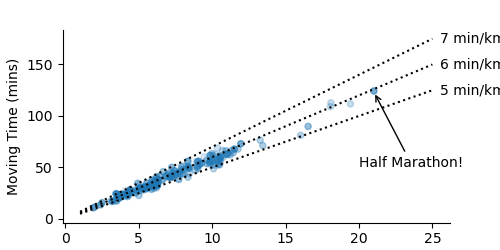
I recently ran my first half marathon! I’m also signed up for a full marathon in October. 😬

Anyway, to celebrate the occasion and because I have now have a reason to think about how fast I might run a particular distance. I had a look at my historical run data. There’s a great website called statshunter that you can authorise to Strava and from which you can download a little csv of all your runs. The first logical thing I could think to do is to see how fast I tend to run different distances.

So it's pretty much a straight line. This is telling me what I kinda already knew: I'm comfortable running between 5 and 7 mins/km and that's basically how fast I always run regardless of distance.

A friend lent me a huge running book which I’m going to dig through more but I suspect one of the conclusions will be a bit obvious: I could run those shorter distances a lot faster.

That same friend also lent me a heart rate watch which I’ve been playing with. So the next thing I want to learn about is what type of heart rates you should target when you train for a particular event.

Code:

from matplotlib import pyplot as plt
import numpy as np
from datetime import datetime
import pandas as pd

runs = pd.read_csv("runs.csv", parse_dates = ["Date"]) # Get this from statshunter.com

f, (ax2, ax) = plt.subplots(nrows=2, figsize = (5,5), sharex = True,
                           gridspec_kw = dict(height_ratios = (1,2)))

ax.set(ylabel = "Moving Time (mins)", xlabel = "Distance (km)")

x = runs["Distance (m)"].values/1e3
y = runs["Moving time"].values/60

dists = np.linspace(1, 25, 2)
for i in [5,6,7]:
    mins_per_km = i * dists
    ax.plot(dists, mins_per_km, color = "black", linestyle = "dotted", label = f"{i} min/km")
    ax.text(25.5, 25*i, f"{i} min/km", va = "center")

ax.annotate("Half Marathon!", (x[0], y[0]-1), (20, 50), arrowprops = dict(arrowstyle = "->"))

ax.scatter(x, y, s=20, alpha = 0.6*fade_out_by_date(runs["Date"]))
for a in [ax, ax2]: a.spines[['right', 'top']].set_visible(False)

ax2.hist(x, bins = 30, alpha = 0.5)
ax2.set(yticks=[], ylabel = "Frequency Density")

f.savefig("time_vs_distance_plus_hist.svg", transparent=True)