Direct Random Sampling

In almost any computer simulation the ultimate source of randomness is a stream of (close to) uniform, uncorrelated bits generated from a pseudo random number generator. A direct sampling method takes such a source and outputs uncorrelated samples from the target distribution. The fact they are uncorrelated is key as we’ll see later. Examples of direct sampling methods range from the trivial: take n random bits to generate integers uniformly between 0 and \(2^n\) to more complex methods such as inverse transform sampling and rejection sampling  [1].

In physics the distribution we usually want to sample from is the Boltzmann probability over states of the system \(S\): \[ \begin{aligned} p(S) &= \frac{1}{\mathcal{Z}} e^{-\beta H(S)}, \\ \end{aligned} \] where \(\mathcal{Z} = \sum_S e^{-\beta H(S)}\) is the normalisation factor and ubiquitous partition function. In principle we could directly sample from this, for a discrete system there are finitely many choices. We could calculate the probability of each one and assign each a region of the unit interval which we could then sample uniformly from.

However, if we actually try to do this we will run into two problems, we can’t calculate \(\mathcal{Z}\) for any reasonably sized systems because the state space grows exponentially with system size. Even if we could calculate \(\mathcal{Z}\), sampling from an exponentially large number of options quickly become tricky. This kind of problem happens in many other disciplines too, particularly when fitting statistical models using Bayesian inference  [2].

MCMC Sampling

So what can we do? Well it turns out that if we are willing to give up in the requirement that the samples be uncorrelated then we can use MCMC instead.

MCMC defines a weighted random walk over the states \((S_0, S_1, S_2, ...)\), such that in the long time limit, states are visited according to their probability \(p(S)\).  [3–5].   [6]

\[\lim_{i\to\infty} p(S_i) = P(S).\]

In a physics context this lets us evaluate any observable with a mean over the states visited by the walk. \[\begin{aligned} \langle O \rangle & = \sum_{S} p(S) \langle O \rangle_{S} = \sum_{i = 0}^{M} \langle O\rangle_{S_i} + \mathcal{O}(\tfrac{1}{\sqrt{M}}).\\ \end{aligned}\]

The samples in the random walk are correlated so the samples effectively contain less information than \(N\) independent samples would. As a consequence the variance is larger than the \(\langle O^2 \rangle - \langle O\rangle^2\) form it would have if the estimates were uncorrelated. Methods of estimating the true variance of \(\langle O \rangle\) and decided how many steps are needed will be considered later.

Implementation of MCMC

In implementation MCMC can be boiled down to choosing a transition function \(\mathcal{T}(S_{t} \rightarrow S_{t+1})\) where \(S\) are vectors representing classical spin configurations. We start in some initial state \(S_0\) and then repeatedly jump to new states according to the probabilities given by \(\mathcal{T}\). This defines a set of random walks \(\{S_0\ldots S_i\ldots S_N\}\).

In pseudo-code one could write the MCMC simulation for a single walker as:

# A skeleton implementation of MCMC
current_state = initial_state

for i in range(N_steps):
    new_state = sampleT(current_state) 
    states[i] = current_state

Where the sampleT function samples directly from the transition function \(\mathcal{T}\).

If we run many such walkers in parallel we can then approximate the distribution \(p_t(S; S)\) which tells us where the walkers are likely to be after they’ve evolved for \(t\) steps from an initial state \(S_0\). We need to carefully choose \(\mathcal{T}\) such that the probability \(p_t(S; S_0)\) approaches the distribution of interest. In this case the thermal distribution \(P(S; \beta) = \mathcal{Z}^{-1} e^{-\beta F(S)}\).

Global and Detailed balance equations

We can quite easily write down the properties that \(\mathcal{T}\) must have in order to yield the correct target distribution. Since we must transition somewhere at each step, we first have the normalisation condition that \[\sum\limits_S \mathcal{T}(S' \rightarrow S) = 1.\]

Second, let us move to an ensemble view, where rather than individual walkers and states, we think about the probability distribution of many walkers at each step. If we start all the walkers in the same place the initial distribution will be a delta function and as we step the walkers will wander around, giving us a sequence of probability distributions \(\{p_0(S), p_1(S), p_2(S)\ldots\}\). For discrete spaces we can write the action of the transition function on \(p_i\) as a matrix equation

\[\begin{aligned} p_{i+1}(S) &= \sum_{S' \in \{S\}} p_i(S') \mathcal{T}(S' \rightarrow S). \end{aligned}\]

This equation is essentially just stating that total probability mass is conserved as our walkers flow around the state space.

In order that \(p_i\) converges to our target distribution \(p\) in the long time limit, we need the target distribution to be a fixed point of the transition function

\[\begin{aligned} P(S) &= \sum_{S'} P(S') \mathcal{T}(S' \rightarrow S). \end{aligned} \] Along with some more technical considerations such as ergodicity which won’t be considered here, global balance suffices to ensure that a MCMC method is correct  [7].

A sufficient but not necessary condition for global balance to hold is called detailed balance:

\[ P(S) \mathcal{T}(S \rightarrow S') = P(S') \mathcal{T}(S' \rightarrow S). \]

In practice most algorithms are constructed to satisfy detailed rather than global balance, though there are arguments that the relaxed requirements of global balance can lead to faster algorithms  [8].

The goal of MCMC is then to choose \(\mathcal{T}\) so that it has the desired thermal distribution \(P(S)\) as its fixed point and converges quickly onto it. This boils down to requiring that the matrix representation of \(T_{ij} = \mathcal{T}(S_i \to S_j)\) has an eigenvector with entries \(P_i = P(S_i)\) with eigenvalue 1 and all other eigenvalues with magnitude less than one. The convergence time depends on the magnitude of the second largest eigenvalue.

The choice of the transition function for MCMC is under-determined as one only needs to satisfy a set of balance conditions for which there are many solutions  [7]. The standard choice that satisfies these requirements is called the Metropolis-Hastings algorithm.

The Metropolis-Hastings Algorithm

The Metropolis-Hastings algorithm breaks the transition function into a proposal distribution \(q(S \to S')\) and an acceptance function \(\mathcal{A}(S \to S')\). \(q\) must be a function we can directly sample from, and in many cases takes the form of flipping some number of spins in \(S\), i.e., if we are flipping a single random spin in the spin chain, \(q(S \to S')\) is the uniform distribution on states reachable by one spin flip from \(S\). This also gives the symmetry property that \(q(S \to S') = q(S' \to S)\).

The proposal \(S'\) is then accepted or rejected with an acceptance probability \(\mathcal{A}(S \to S')\), if the proposal is rejected then \(S_{i+1} = S_{i}\). Hence:

\[\mathcal{T}(S\to S') = q(S\to S')\mathcal{A}(S \to S').\]

The Metropolis-Hasting algorithm is a slight extension of the original Metropolis algorithm which allows for non-symmetric proposal distributions \(q(S\to S') \neq q(S'\to S)\). It can be derived starting from detailed balance  [6]:

\[ P(S)\mathcal{T}(S \to S') = P(S')\mathcal{T}(S' \to S), \]

inserting the proposal and acceptance function

\[ P(S)q(S \to S')\mathcal{A}(S \to S') = P(S')q(S' \to S)\mathcal{A}(S' \to S), \]

rearranging gives us a condition on the acceptance function in terms of the target distribution and the proposal distribution which can be thought of as inputs to the algorithm

\[ \frac{\mathcal{A}(S \to S')}{\mathcal{A}(S' \to S)} = \frac{P(S')q(S' \to S)}{P(S)q(S \to S')} = f(S, S'). \]

The Metropolis-Hastings algorithm is the choice

\[ \begin{aligned} \label{eq:mh} \mathcal{A}(S \to S') = \min\left(1, f(S,S')\right), \end{aligned} \] for the acceptance function. The proposal distribution is left as a free choice.

Noting that \(f(S,S') = 1/f(S',S)\), we can see that the MH algorithm satisfies detailed balance by considering the two cases \(f(S,S') > 1\) and \(f(S,S') < 1\).

By choosing the proposal distribution such that \(f(S,S')\) is as close as possible to one, the rate of rejections can be reduced and the algorithm sped up. This can be challenging though, as getting \(f(S,S')\) close to 1 would imply that we can directly sample from a distribution very close to the target distribution. As MCMC is usually applied to problems for which there is virtually no hope of sampling directly from the target distribution, it’s rare that one can do so approximately.

When the proposal distribution is symmetric as ours is, it cancels out in the expression for the acceptance function and the Metropolis-Hastings algorithm is simply the choice

\[ \mathcal{A}(S \to S') = \min\left(1, e^{-\beta\;\Delta F}\right), \]

where \(F\) is the overall free energy of the system, including both the quantum and classical sector.

To implement the acceptance function in practice we pick a random number in the unit interval and accept if it is less than \(e^{-\beta\;\Delta F}\):

# An implementation of the standard MH algorithm
current_state = initial_state

for i in range(N_steps):
    new_state = proposal(current_state)
    df = free_energy_change(current_state, new_state, parameters)

    if uniform(0,1) < exp(-beta * df):
        current_state = new_state
        
    states[i] = current_state

Two Step Trick

Our method already relies heavily on the split between the classical and quantum sector to derive a sign problem free MCMC algorithm but it turns out that there is a further trick we can play with it. The free energy term is the sum of an easy to compute classical energy and a more expensive quantum free energy, we can split the acceptance function into two in such a way as to avoid having to compute the full exact diagonalisation some of the time:

# Our two step MH implementation for models with classical and quantum energy terms
current_state = initial_state

for i in range(N_steps):
    new_state = proposal(current_state)

    df_classical = classical_free_energy_change(current_state, new_state, parameters)
    if exp(-beta * df_classical) < uniform(0,1):
        f_quantum = quantum_free_energy(current_state, new_state, parameters)
    
        if exp(- beta * df_quantum) < uniform(0,1):
          current_state = new_state
    
        states[i] = current_state
    

As discussed in the main text, for the model parameters used, we find that with our new scheme the matrix diagonalisation is skipped around 30% of the time at \(T = 2.5\) and up to 80% at \(T = 1.5\). We observe that for \(N = 50\), the matrix diagonalisation, if it occurs, occupies around 60% of the total computation time for a single step. This rises to 90% at N = 300 and further increases for larger N. We therefore get the greatest speedup for large system sizes at low temperature where many prospective transitions are rejected at the classical stage and the matrix computation takes up the greatest fraction of the total computation time. The upshot is that we find a speedup of up to a factor of 10 at the cost of very little extra algorithmic complexity.

This modified scheme has the acceptance function \[\mathcal{A}(a \to b) = \min\left(1, e^{-\beta \Delta H_s}\right)\min\left(1, e^{-\beta \Delta F_c}\right).\]

We can show that this satisfies the detailed balance equations as follows. Defining \(r_c = e^{-\beta H_c}\) and \(r_q = e^{-\beta F_q}\) our target distribution is \(\pi(a) = r_c r_q\). This method has \(\mathcal{T}(a\to b) = q(a\to b)\mathcal{A}(a \to b)\) with symmetric \(p(a \to b) = \pi(b \to a)\) and \(\mathcal{A} = \min\left(1, r_c\right) \min\left(1, r_q\right)\)

Substituting this into the detailed balance equation gives: \[\mathcal{T}(a \to b)/\mathcal{T}(b \to a) = \pi(b)/\pi(a) = r_c r_q.\]

Taking the LHS and substituting in our transition function: \[\begin{aligned} \mathcal{T}(a \to b)/\mathcal{T}(b \to a) = \frac{\min\left(1, r_c\right) \min\left(1, r_q\right)}{ \min\left(1, 1/r_c\right) \min\left(1, 1/r_q\right)},\end{aligned}\]

which simplifies to \(r_c r_q\) as \(\min(1,r)/\min(1,1/r) = r\) for \(r > 0\).

Autocorrelation Time

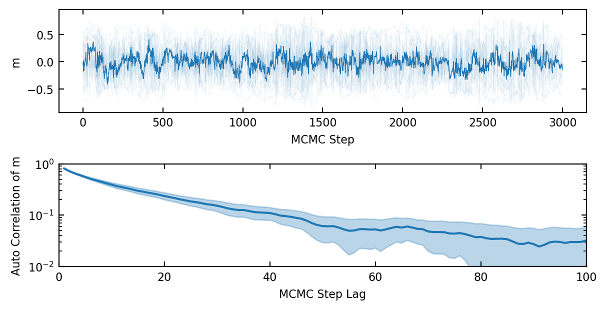
At this stage one might think we are done. We can indeed draw independent samples from our target Boltzmann distribution by starting from some arbitrary initial state and doing \(k\) steps to arrive at a sample. These are not, however, independent samples. In fig. 1 it is already clear that the samples of the order parameter \(m\) have some autocorrelation because only a few spins are flipped each step. Even when the number of spins flipped per step is increased that it can be an important effect near the phase transition. Let’s define the autocorrelation time \(\tau(O)\) informally as the number of MCMC samples of some observable O that are statistically equal to one independent sample or equivalently as the number of MCMC steps after which the samples are correlated below some cut-off, see ref.  [9]. The autocorrelation time is generally shorter than the convergence time so it therefore makes sense from an efficiency standpoint to run a single walker for many MCMC steps rather than to run a huge ensemble for \(k\) steps each.

Once the random walk has been carried out for many steps, the expectation values of \(O\) can be estimated from the MCMC samples \(S_i\): \[ \langle O \rangle = \sum_{i = 0}^{N} O(S_i) + \mathcal{O}(\frac{1}{\sqrt{N}}). \]

The samples are correlated so the N of them effectively contains less information than \(N\) independent samples would, in fact roughly \(N/\tau\) effective samples. As a consequence the variance is larger than the \(\langle O^2 \rangle - \langle O \rangle ^2\) form it would have if the estimates were uncorrelated. There are many methods in the literature for estimating the true variance of \(\langle O \rangle\) and deciding how many steps are needed but my approach has been to run a small number of parallel chains, which are independent, in order to estimate the statistical error produced. This is a slightly less computationally efficient because it requires throwing away those \(k\) steps generated before convergence multiple times but it is conceptually simple.

Tuning the proposal distribution

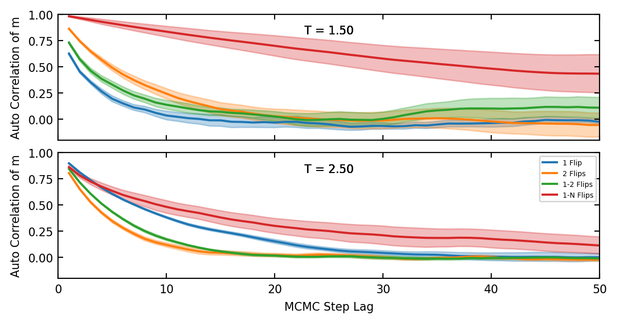
Now we can discuss how to minimise the autocorrelations. The general principle is that one must balance the proposal distribution between two extremes. Choose overly small steps, like flipping only a single spin and the acceptance rate will be high because \(\Delta F\) will usually be small, but each state will be very similar to the previous and the autocorrelations will be high too, making sampling inefficient. On the other hand, overlay large steps, like randomising a large portion of the spins each step, will result in very frequent rejections, especially at low temperatures.

I evaluated a few different proposal distributions for use with the FK model.

1. Flipping a single random site
2. Flipping N random sites for some N
3. Choosing n from Uniform(1, N) and then flipping n sites for some fixed N.
4. Attempting to tune the proposal distribution for each parameter regime.

Fro fig. 2 we see that even at moderately high temperatures \(T > T_c\) flipping one or two sites is the best choice. However, for some simulations at very high temperature flipping more spins is warranted.

Next Section: Lattice Generation